Usage
Runmanager is the primary means of defining and managing the set of experiment parameters (global variables - see §5.1.3) used in the labscript experiment logic. Runmanager also handles the creation of each hdf5 shot file, and the invocation of labscript via the execution of a user specified labscript experiment logic file.
The graphical interface
We believe that the manipulation of parameters, along with controls for producing shots, are best implemented in a graphical interface. Critical information on the current runmanager configuration, along with controls for generating new shots, are located in a always visible toolbar at the top of the runmanager interface. These comprise (as labelled in Fig. 2):
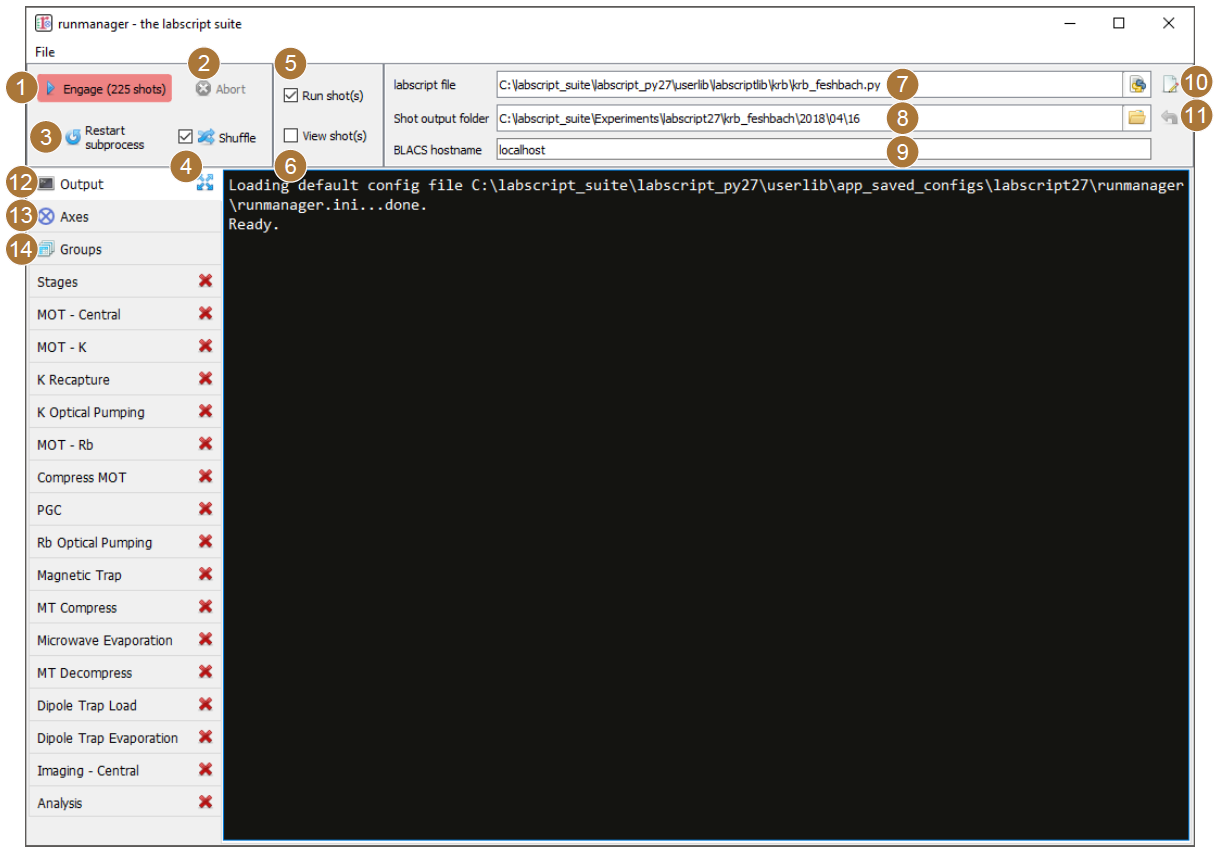
Fig. 2 The runmanager graphical interface with the main controls labelled as per the below text. The ‘output’ tab is currently shown.
The engage button: This begins production of the appropriate number of shot files. The number of shot files that will be produced is displayed prominently in the button text so that any mistakes made when defining the parameter space scan can be quickly corrected prior to beginning shot generation. This button can also be ‘clicked’ via the F5 key on a keyboard.
The abort button: This stops the production of shot files prematurely.
The restart subprocess button: Primarily for debugging and for use during labscript development, this button restarts the subprocess that manages the execution of the labscript experiment logic file, which in turn generates and stores hardware instructions inside the hdf5 file (see Shot creation).
The shuffle checkbox: This checkbox controls the global setting for whether parameter space scans are shuffled or not. This is a tri-state checkbox (all-some-none) displaying the current shuffle state on the axes tab. Clicking the checkbox will overwrite the state of each entry on the axes tab with the new state of the global checkbox. For more details, see Parameter space scans.
The run shots checkbox: If ticked prior to clicking the engage button, shot files will be sent immediately to the BLACS queue once the hardware instructions have been generated by labscript.
The view shots checkbox: If ticked prior to clicking the engage button, shots will be sent to runviewer once the hardware instructions have been generated by labscript. Runviewer is assumed to be running locally, and will be launched if it is not already running once the first hdf5 file has been generated.
The labscript file: The Python file containing the experiment logic to be compiled into hardware instructions (see labscript).
The shot output folder: The location to store the hdf5 shot files. By default, the location in specified by the combination of a value in the laboratory PC configuration file (see labconfig), the name of the experiment logic Python file and the current date. The location automatically updates, at midnight, to a new folder for the day provided the folder location is left as the default.
The BLACS hostname: The network hostname of the PC the hdf5 shot files are to be sent to if the ‘run shots’ checkbox is ticked. It is expected that BLACS is running on the specified PC, and that network access (including firewalls and other network access controls) is configured appropriately.
The open in editor button: This button open the specified labscript experiment logic file in the text editor specified in the laboratory PC configuration file (see labconfig in the glossary).
The reset shot output folder button: This button resets the shot output folder to the default. This will re-enable the auto incrementation of the folder (based on the current date), which is disabled for custom locations.
These controls provide rapid access to the key functionality of runmanager (creating and distributing shot files) at all times, making for an efficient workflow. The rest of the runmanager interface exists within a set of tabs. The first 3 tabs contain further runmanager specific controls:
The output tab: This tab contains the terminal output of the shot creation process including the terminal output produced during the execution of the labscript experiment logic file. For example, Python
printstatements included in the experiment logic code will appear here during shot creation. This makes it easy to debug the experiment logic code using simple methods common to general purpose programming. Warnings and error messages generated by the labscript API also appear here in red text, so that any issues are immediately noticed and can be actioned. As this output is useful for debugging purposes, we allow the tab to be ‘popped out’ into a separate window so it can be visible at the same time as another tab (to avoid the need to frequently switch between the output and the tab containing the global variable(s) you are currently modifying).The axes tab: This tab allows the user to control the iteration order of the parameters in the defined parameter space (see Fig. 3). The length of each axis of the parameter space is displayed, as is a shuffle checkbox for determining whether the points along that axis should be shuffled before the parameter space is expanded into the set of shots to be created. The global shuffle control (see item 4 in this list) is linked to the state of the shuffle checkboxes on the axes tab. This feature, along with the many benefits, is detailed further in Parameter space scans (see feature 3 and the paragraphs following).
The groups tab: This tab manages the hdf5 files that store the globals (see Fig. 4). Further details on managing global variables will be discussed in Managing global variables.
These tabs are then followed by an arbitrary number of tabs containing sets of global variables, which will be discussed further in Managing global variables.
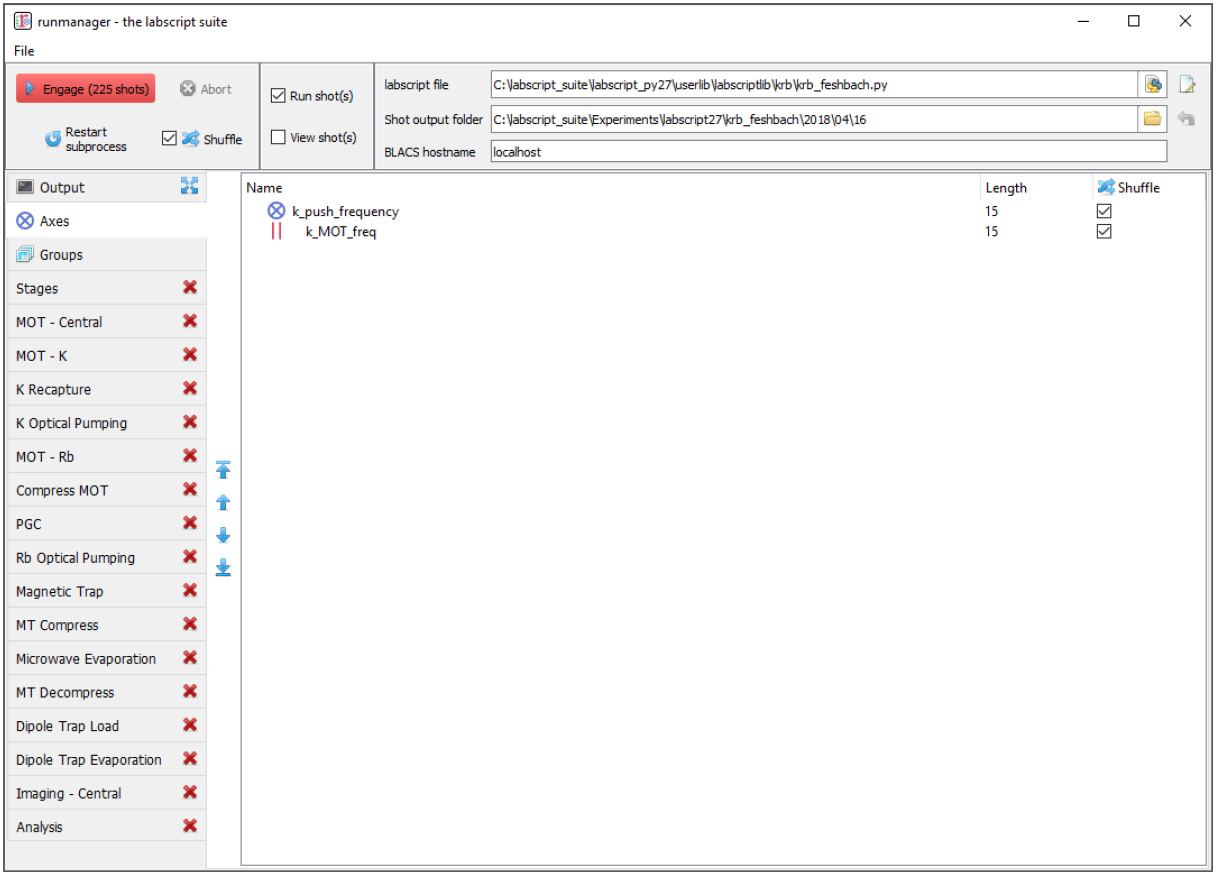
Fig. 3 The ‘Axes’ tab of runmanager. This tab displays a list of all global variables (indicated by the blue outer product icon) or groups of global variables (indicated by the icon with red parallel bars) that form axes of the parameter space that will be scanned over (see item 13 and Parameter space scans for further details). The order of the axes can be changed using the controls to the left of the list, which sets the order in which the outer product of the axes is performed (when generating the shot files).
In addition to this, runmanager can save and restore the entire GUI state via the relevant menu items in the ‘File’ menu. This allows rapid switching between different types of experiment logic and/or globals files. [2] This is particularly useful for shared experiment apparatuses, where different users want to run different experiments, and for the cases where a user wishes to rapidly switch between one of more diagnostic configurations they have previously saved.
Managing global variables
Runmanager provides a simple interface for grouping and modifying global variables. As mentioned previously, the ‘groups’ tab in runmanager handles creating and opening the hdf5 files that store the global variables. There are two levels of organisation for global variables:
at the file level (globals can be stored across multiple files, the union of which is used to generate shots), and
groups within each file.
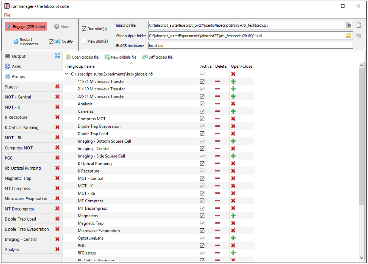
Fig. 4 The ‘Groups’ tab of runmanager. This tab displays the groups of global variables (stored in hdf5 files) that have been loaded into runmanager. From this tab, users can enabled/disable the use of these globals when compiling shots (using the ‘active’ checkboxes) and open/close an editing tab for each group. The editing tabs, when open, are displayed as additional tabs on the left most edge of the runmanager interface. See Managing global variables for further details on managing globals.
Globals groups are created from the ‘groups’ tab in runmanager and can have arbitrary names (including spaces and special symbols). The only requirement is that a group name is unique within its file (it can however have the same name as a group in a different file). Globals within a group are then only used in the creation of shots if the ‘active’ checkbox for the group is checked on the groups tab (see Fig. 4). This provides a simple way of switching between different groups of globals, allowing labs to maintain a common set of parameters for their experiments as well as individual parameter sets for specific users and/or experiments. For example, rather than modifying a set of globals in a group, a user could instead deactivate the group containing those globals, and instead ask runmanager to pull those globals from a separate file.
Each group of globals can be opened for editing in a new tab. We provide columns
for the global name, value and units. The global name must be a valid Python variable
name, and must not conflict with any member of the pylab library, python keywords,
or existing items in the Python __builtin__ module. This ensures that it can be injected
into the labscript experiment logic (see labscript) without conflicting with existing Python
functionality. The global name must also be unique across all active groups, as global
groups are joined into a single set before passing the globals into the labscript experiment
logic.
The value of a global can be any Python expression (including the use of functions from the numpy module), that evaluates to a datatype supported by hdf5, such as, but not limited to:
a number:
1234or780e-9,a string:
'N_atoms',a list or numpy array (which will be treated as an axis of a parameter space to scan, where the global variable will contain only one of the elements of the list or array in each shot):
[1, 2, 3]orarray([1, 2, 3]),a tuple (which despite being list like, will not be treated as an axis of a parameter space to scan and will instead be passed into labscript as the tuple specified):
(1, 2, 3),a Boolean:
TrueorFalsean equation:
1+2a Python inbuilt, or numpy, function call that returns a valid value:
linspace(0, 10, 10),an expression that references another defined global variable by name (the value of this global variable is used in its place):
2*other_globalorlinspace(0, 10, other_global),a Boolean expression:
(other_global1 and other_global2)or(other_global3 == 7)or(other_global4), orany of the above plus a Python comment:
780e-9 #This was previously 781e-9.
As these expressions can become quite complex (see Fig. 5), the tooltip for the value cells displays the evaluated result of the Python expression. The value cell is also colour coded to the successful evaluation of the expression, so that mistakes can be easily identified (see Fig. 6).
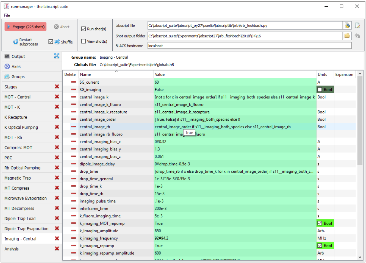
Fig. 5 An example of complex global variables that utilise Python expressions to define their value.
Note, for example the drop_time global variable, whose full expression is shown below. The
drop_time used is always drawn from one of three global variables, but the global variable selected
is determined by a separate global variable (a Boolean) and may contain a list of drop times if
the user wishes to image multiple species. In the case of the expression generating a list, this
global becomes an axis of a parameter space, running two shots for every other data point in the
parameter space (one shot to image each of the two species our experiment supports). Such an
expression could not be defined within experiment logic as parameter spaces must be defined within
runmanager, not labscript. In order to simplify the view of globals with complex expressions, the
tooltip (shown for the central_image_rb global) shows the value(s) the global will take in the next
compiled shot(s).
[ drop_time_rb if x else drop_time_k for x in central_image_order ] if
s11__imaging_both_species else ( drop_time_k if central_image_k == True
else ( drop_time_rb if central_image_rb == True else drop_time_general))
The units of the global are not currently passed into the labscript experiment logic
code, but are a way to provide context to the user within runmanager. For example, if the
labscript experiment logic multiplied a global variable for a frequency by 1e6 everywhere
it was used (or the keyword argument units="MHz" was used everywhere), then you could
type ‘MHz’ into the units column of runmanager so that a later user would know that the
global was expected to be of that magnitude and would not accidentally enter it in kHz
or Hz. In addition to this, globals whose values are explicitly specified as either True or
False have their units automatically set to ‘Bool’, a checkbox is placed in the units column
for easy toggling, and the units cell is colour coded to this checkbox for easy observation
of the state. We frequently use this functionality to enable/disable various stages of our
experiment logic file (see Fig. 7).
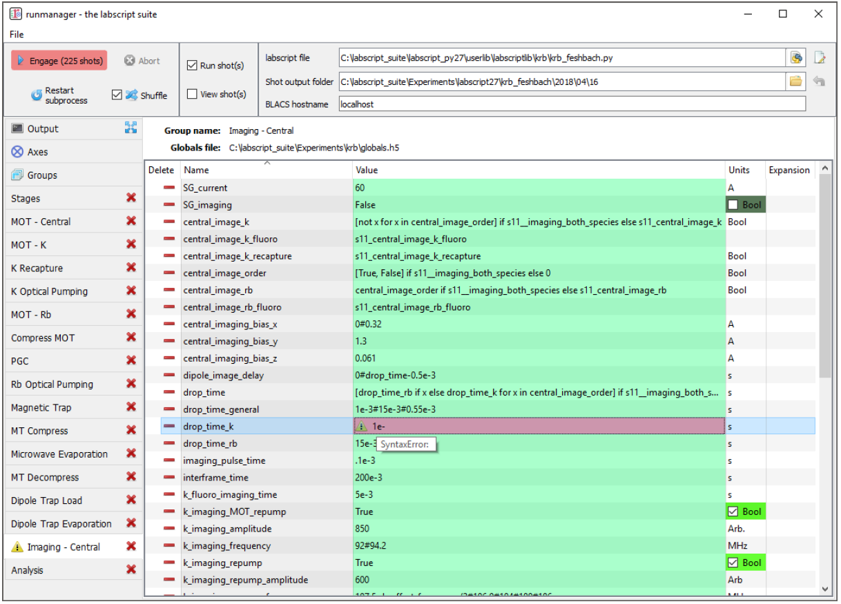
Fig. 6 An example of an evaluation error in a global variable. The user is notified of the error in two places: an icon appears next to the tab name and the global in question is highlighted in red. The tooltip displays the cause of the error, in this case a Python syntax error.
While we recommend storing globals in a dedicated set of files, the storage format for the globals is identical to that in any shot, which allows a user to easily load in globals from existing shots (even ones that have been executed and analysed). However, once pointed at an existing shot file, any modification to globals will modify that shot file, thus partially destroying the complete record of the experiment. [3] Thus, we encourage this feature to only be used for the cases where you wish to look at the globals from an old shot or where you wish to use the globals, without modification, to compile new shots.
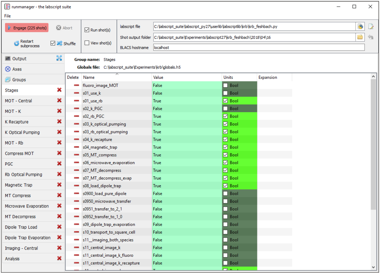
Fig. 7 An example of how a labscript experiment can be parameterised by a series of Boolean global variables. Here we split up the production of a BEC into several stages. We name each global with a prefix that increments in order to keep the globals in an appropriate sort order. Runmanager detects the Boolean type of the global, and provides a simple checkbox toggle in the units column, By using these global variables in our labscript experiment logic file, as the Boolean expression for an if statement, we can quickly turn on/off various stages of the BEC production process (which is very useful when debugging or optimising the BEC production process).
Parameter space scans
One of the key features of runmanager (and critical goals of our scientific control system) is the ability to easily automate the traversal of a large parameter space, an increasingly important requirement for performing modern ultracold atom experiments. Runmanager provides four features for managing parameter space scans:
The automatic detection of global variables that are defined as a list. [4] Such globals are labelled ‘outer’ in the expansions column as all such globals will be combined, via an outer product, into the parameter space to be scanned. The number of shots to be generated, which is simply the product of the lengths of all ‘outer’ product globals, is displayed next to the engage button.
The ability to define what we term ‘zip groups’ after the Python function
zip. Two (or more) globals (specified as lists) can be grouped together so that they iterate through values in lockstep. In this instance, the zip group is used as a single axis of the outer product rather than one axis for each global.The third feature is the ability to define the order in which the axes of the parameter space are iterated over when producing individual shots (see the ‘Axes’ tab discussed previously in The graphical interface).
The ability to randomly shuffle the order of values within each global (or zip group) defined as a list. This can be done on a per global basis or on the entire set of shots that spans the defined parameter space.
These features provide a powerful basis for performing complex experiments.
Consider the following example. Many of the early stages of BEC production (for instance the MOT or magnetic trap stages) should be optimised for best phase-space density. Phase space density is calculated from several parameters; the most important being atom number and atom cloud temperature. While atom number can be easily measured from an absorption image from a single shot, temperature is most commonly determined from analysing the result of multiple shots. In this case, the drop time (the time between releasing the atoms from the trap and taking the absorption image) is varied for each shot and the temperature determined by fitting to the linearised relationship between atom cloud size and drop time. Already, it can be seen that measuring the phase space density for a single set of parameters requires several shots, which can be easily automated via the feature 1 described above.
Now consider the optimisation of MOT or magnetic trap parameters. Many of these are
coupled and can not be independently optimised. As such, it is preferable to optimise two
or three variables at once, measuring the phase-space density at each point to determine the
optimal set of parameters. Such a parameter space typically takes several hours to complete
due to the large number of shots that must be run. A BEC apparatus is likely to undergo
systematic drifts during this time, which may invalidate the results. However, with careful
thought, features 3 and 4 can be used to counteract this. For example, systematic drift will
effect the linearity of the data when determining temperature, especially if the acquisition
of each data point is separated by a significant period of time. However, by defining the
drop time to be the inner most item of the outer product, you ensure that all shots needed
to determine the phase-space density for a single set of MOT parameters are executed as
close together in time as possible. Shuffling the order of the drop time then eliminates short
term systematic drift, as does separately shuffling the order of the values in each remaining
axes of the outer product (the MOT parameters). If long term systematic drifts need to
be quantified, then an additional axes to the outer product can be added at the outer most
layer in order to repeat each of the shots a prescribed number of times (by defining an
additional ‘dummy’ global variable as range(N) where N is the number of times to repeat
each shot).
While the above example may seem complicated, runmanager makes it trivial to implement. A user simply defines the list of values to scan over for each parameter, sets the order in which the outer product should use each axis, and specifies whether the values for each axis should be shuffled. Once done, clicking the engage button generates the sequence of shots and sends them to BLACS to be executed on the experiment.
Evaluation of globals
All global variable expressions are automatically evaluated after a change to any global variable. This serves to both update the tooltip with the result of the expression, detect axes of a parameter space to scan (and group them into zip groups if appropriate) and warn the user of any errors during the evaluation of the globals. As discussed previously, runmanager allows these global variable expressions to reference other global variables. This allows a user to maintain a record of a set of parameters, and all relevant quantities derived from one or more of those parameters, without ever storing a parameter more than once. This ensures that important quantities need not be derived (from globals) in the labscript experiment logic script, and that they are accessible directly during the analysis stage (see lyse).
To implement this, we take advantage of the Python built-in function exec which not
only evaluates a string containing a Python expression, but can do so from within a controlled
namespace. This has a two-fold benefit. The first is that it allows us to provide
access to a specific set of functions that can be used from within the Python expressions
(such as numpy functions like linspace). The second is that it allows us to keep track of the
relationship between global variables, which is critical for both descriptive error messages
and automatically detecting which globals should be combined into a zip groups.
The Python exec function is given access to a namespace to work in via an optional
argument in the form of a dictionary. Keys and values in this dictionary correspond to
variable names in the namespace and their associated values respectively. Rather than
using a native Python dictionary for the namespace, we subclass the Python dictionary
and override the built-in dictionary method for looking up entries in the dictionary. When
combined with exec, this translates to our dict subclasses tracking each time the exec
function requests the value of a variable in the namespace. This then provides us with a
mapping of each global variable, and the names of global variables that it depends on. In
order to resolve both the order in which global variable expressions are evaluated in, and
detection of any recursive relationships, we begin by evaluating all global expressions and
then recursively re-evaluate the set of globals that did not evaluate in the previous iteration.
The first iteration will evaluate any (correctly defined) independent globals, and subsequent
iterations will then be able to evaluate globals that depend on other globals (once those
other globals have been evaluated by a previous iteration).
The hierarchy of global interdependencies is then used to determine automatic zip group names, which are based on the name of the global in the hierarchy that does not depend on any other. If a global depends on multiple other globals, then the zip group name is chosen semi-randomly based on the order of the items in the Python dictionary (which depends on a hash of the dictionary key names and the size of the dictionary). However, it is of course always possible to overwrite the automatic zip group name with something else should our algorithm choose incorrectly.
We believe that this complex evaluation of global variables is only possible due to the use of an interpreted language that has tools for parsing its own syntax. As such, the choice of Python as our programming language has allowed us to implement extremely useful, advanced features that might otherwise be too difficult to produce in more low level languages such as C++.
Shot creation
The internal process for generating shot files is quite complex. This is primarily motivated by the desire for modularity (for example, to separate shot file generation from hardware instruction generation) and the desire for robustness. As runmanager ultimately initiates the execution of user code (the labscript experiment logic file), there is a risk that problems in the user code could crash runmanager. We mitigate this by using a multi-process architecture.
We originally spawned a new Python process for each shot (in order to guarantee the internal state of labscript was fresh). However the time required to start a Python process (especially on Windows) was a considerable fraction of the entire shot generation time. As such we now use a single, long-lived, Python process and clean-up the internal state of labscript and Python explicitly after each shot.
To generate shot files, runmanager:
Re-evaluates all globals (see Evaluation of globals). This both determines the number of shots to produce, and generates the evaluated set of global variables for each shot.
The globals are then written to hdf5 files, one file for each shot. We also write the unevaluated globals into every hdf5 file, in order to provide a complete record of the experiment (the unevaluated globals contain information about the parameter space that is not available when looking at the single point of parameter space in the evaluated globals of a single shot file).
In a thread (in order to keep the GUI responsive), we iterate over the set of files and send their file paths to a long-running subprocess (launched by runmanager at startup) that is used to execute labscript code in an isolated environment. We call this process the ‘compilation subprocess’.
The subprocess, which has the labscript API imported, calls an initialisation method to inform the labscript API of the hdf5 file to write hardware instructions to.
The subprocess loads the global variables from runmanager into the
__builtin__dictionary.The subprocess then executes the labscript experiment logic file (using the Python function
exec) in an isolated namespace, which invokes the labscript API via the users experiment logic and generates the required hardware instructions and saves them in the hdf5 file. Terminal output (for example,printstatements) are sent back to the parent runmanager process and placed in the output tab.The subprocess restores the
__builtin__dictionary to its original state to prevent globals from polluting subsequent shots. A clean-up method from the labscript API is also called so that the internal state of the labscript Python module is also reset.
Once shot files are created, the file paths are sent to runviewer or BLACS, as determined by the checkboxes in the runmanager GUI, for viewing and/or executing the shots respectively. This architecture also has several unrealised benefits:
If the need arose, we could easily parallelise the generation of hardware instructions by instantiating multiple instances of the compilation subprocess.
We could use runmanager as a generic parameter (space) management software by replacing the compilation subprocess with something else. For example, runmanager could be used to manage parameters for simulations, producing one shot file per simulation to be run in the same way we do for real experiments. These files could then be sent to a scheduling program (like BLACS) that feeds them to the simulation software.
Footnotes